flowchart LR
    subgraph ETL ["Traditional ETL"]
        E1["Source"] --> E2["Transform Engine"] --> E3["Load"] --> E4["Data Warehouse"]
    end

    subgraph ELT ["Modern ELT (Today)"]
        L1["Source"] --> L2["Load Raw"] --> L3["Data Warehouse"] --> L4["Transform In-Place"]
    end

    classDef source fill:#0057b8,color:#fff,stroke:#003d82
    classDef transform fill:#d97706,color:#fff,stroke:#b45309
    classDef warehouse fill:#01065c,color:#fff,stroke:#000940

    class E1,L1 source
    class E2,L4 transform
    class E4,L3 warehouse
Module 1: Data Engineering Fundamentals
ETL, medallion, and the NYC Taxi dataset
![]()
![]()
![]()
![]()
![]()
Duration: 35 min — Animation (3) · Think & Discuss (8) · Theory (12) · Quiz (3) · Practice (9)
1. Animation
2. Think & Discuss
Situation: Elena proposed Bronze, Silver, Gold. Priya listed five KPI questions but her dashboard is still empty. James will later validate Gold KPIs in SQL; today the team agrees what belongs in each layer before anyone writes pipeline code.
Prompts:
- Why three layers instead of one big table for Marcus?
- What belongs in Silver vs Gold? Give one example column or metric for each.
- Priya asks: When are our peak revenue hours? — which layer do you query?
- ETL vs ELT — would you transform trip data before or after loading into the platform? One reason for your choice.
- Name one criterion you would use to compare Databricks, Snowflake, and dbt — without picking a winner yet.
3. Theory
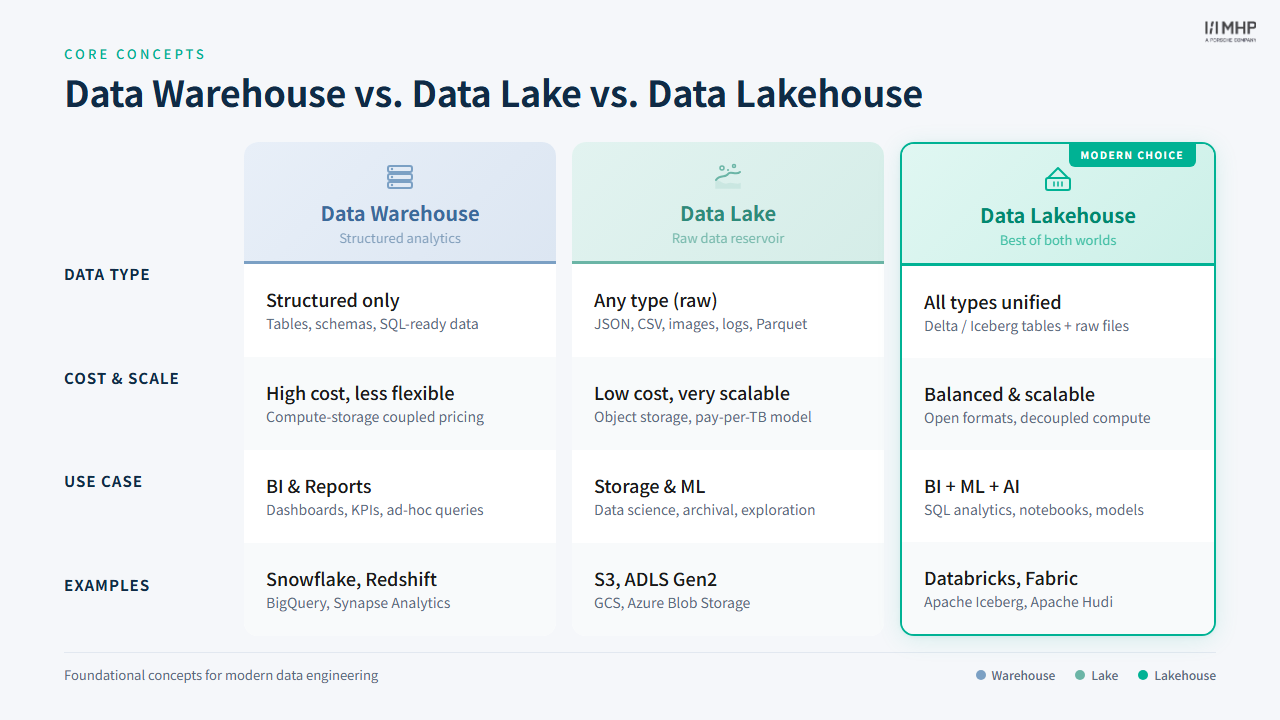
Data Warehouse vs Data Lake vs Data Lakehouse
Understanding these three architectures explains why YellowLine NYC’s new platform uses a lakehouse approach.
| Feature | Data Warehouse | Data Lake | Data Lakehouse |
|---|---|---|---|
| Data types | Structured only | Any format (structured, semi-structured, unstructured) | Any format |
| Primary use | BI & reporting | Data science & ML | BI, ML, and streaming |
| ACID transactions | Yes | No | Yes (via Delta Lake, Iceberg, etc.) |
| Schema | Schema-on-write | Schema-on-read | Schema-on-write with evolution |
| Storage format | Proprietary | Open (Parquet, ORC, JSON, …) | Open (Parquet-based) |
| Cost | High (compute + storage coupled) | Low (cheap object storage) | Low (decoupled compute & storage) |
| BI latency | Low (optimized for SQL) | High (unvalidated data) | Low (optimized metadata layer) |
| ML support | Limited | Full access to raw data | Full — same data for BI and ML |
| Governance | Strong | Weak | Strong (Unity Catalog, Snowflake RBAC) |
Why lakehouse for YellowLine NYC?
A lakehouse gives YellowLine NYC the low-cost, open-format storage of a data lake with the ACID transactions and governance of a data warehouse. Both Databricks and Snowflake now implement this pattern — which is why Elena can run the same medallion layers (Bronze → Silver → Gold) on either platform.
3.1 ETL vs ELT
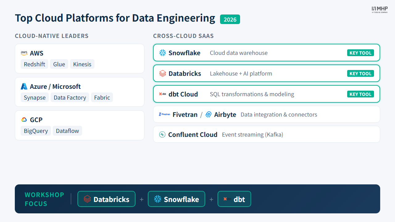
Cloud Platforms for Data Engineering
Before comparing pipeline patterns, let’s survey the cloud platforms where these patterns are implemented.
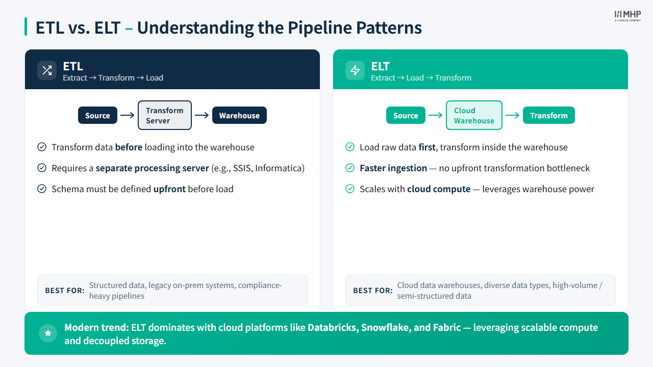
ETL vs ELT
The distinction between ETL and ELT shapes how you design every pipeline in this workshop. In traditional ETL, a separate transformation engine cleanses data before it reaches the warehouse — this made sense when storage was expensive and compute was fixed. Modern cloud platforms invert this: storage is cheap, compute scales elastically, so it is faster and more flexible to load raw data first and transform in-place (ELT).
| ETL | ELT | |
|---|---|---|
| Transform | Before loading | After loading |
| Where | Separate transform engine | Inside the data warehouse |
| Best for | Legacy systems, data cleansing | Cloud DWH, big data, iteration |
| Examples | SSIS, Informatica |
Microsoft Fabric is also an ELT-native SaaS platform — standalone from Azure Synapse, built on Azure infrastructure — that follows the same load-first pattern.
Today’s approach: ELT — we load raw data first, then transform in-place.
Always land raw data first
Even if the source is already clean, always write an exact copy to Bronze before any transformation. This gives you reproducibility (reprocess from raw at any time) and an audit trail (prove what the source looked like at ingestion time). Skipping Bronze is the most common shortcut that creates irreproducible pipelines.
3.2 Medallion Architecture
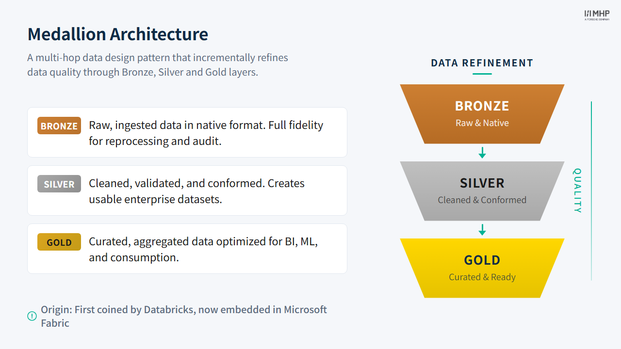
The medallion architecture (also called multi-hop or multi-layer) organizes data into three progressively refined layers. Each layer has a clear contract: what goes in, what transformations are applied, and who consumes the output. This pattern is vendor-neutral — Databricks, Snowflake, and dbt all implement it, each using their own compute engine and syntax. Some organizations use different names — “raw / cleaned / consumption” or “landing / standardised / curated” — but the semantics are identical: raw → trusted → aggregated.
Bronze — Raw Ingestion
- Exact copy of source data — no transformations, no filters
- Metadata added: source file, processing timestamp, partition keys
- Purpose: Reproducibility — you can always reprocess from raw
- Consumer: Silver transformation jobs (never queried directly by analysts)
Silver — Cleaned & Enriched
- Data quality filters applied (nulls, duplicates, outliers removed)
- Column standardization (naming conventions, type casting)
- Derived metrics (trip duration, fare per mile, time features)
- Enrichment (zone lookups joined, descriptive labels added)
- Purpose: Trustworthy, analysis-ready data
- Consumer: Gold aggregations, ML feature tables, ad-hoc analyst queries
Gold — Business KPIs
- Aggregated tables optimized for reporting — one table per KPI or metric group
- Pre-computed for fast dashboard queries (sub-second on Power BI)
- Purpose: Ready for business users, dashboards, and executive reports
- Also feeds: ML feature engineering (tip prediction) and streaming Gold aggregations (optional modules)
Don’t skip Silver
A common mistake is to read directly from Bronze and build Gold KPIs without a cleaning step. Without Silver’s quality filters and standardization, Gold tables silently contain null fares, zero-distance trips, and duplicate rows. The errors compound: a “top routes” KPI built on dirty data looks plausible but is wrong. Always route through Silver — even if the transformation seems simple.
NoteMedallion is vendor-neutral
The layer semantics stay the same across Databricks, Snowflake, and dbt. Databricks also maps medallion hops to Lakeflow Spark Declarative Pipelines (LSDP) — formerly Delta Live Tables.
3.3 Key Takeaways
- Medallion architecture is vendor-neutral — the layer semantics stay the same whether you use Databricks, Snowflake, or dbt
- ELT loads raw data first, then transforms in-place — the dominant pattern for modern cloud data platforms
- Bronze preserves an exact copy of source data for reproducibility and audit
- Silver is where data quality happens — skipping it is the most common cause of silent KPI errors
- The 12 Gold KPIs are the consistent benchmark — all three pipelines produce identical results so you can compare tools fairly
4. Quiz
Quiz: Module 1 — ETL & Medallion Quiz
Before moving on, make sure you can answer:
- What is the key difference between ETL and ELT, and why does this workshop use ELT?
- Name one transformation that belongs in Silver but not in Bronze, and one that belongs in Gold but not Silver.
- Why do we compute the same 12 KPIs in three separate pipelines instead of just one?
5. Practice
NYC Taxi Dataset
We use the NYC Taxi & Limousine Commission trip data — one of the most popular public datasets for data engineering training.
Trip Data (Parquet)
- 3,646,319 yellow taxi trips (October 2024 workshop month —
yellow_tripdata_2024-10.parquet) - 19 columns: pickup/dropoff times, locations, distances, fares, tips, payment types
- Stored as Parquet on Azure ADLS2
Zone Lookup (CSV)
- 265 taxi zones across NYC
- 4 columns: LocationID, Borough, Zone, service_zone
- Used to enrich trip data with human-readable location names
12 Core KPIs
We compute the same 12 KPIs in all three pipelines:
| # | KPI | What It Shows |
|---|---|---|
| 1 | Trips by Hour | Hourly demand patterns |
| 2 | Trips by Day | Weekly patterns |
| 3 | Time of Day Analysis | Morning/Midday/Evening/Night |
| 4 | Top Pickup Zones | Busiest locations |
| 5 | Borough Analysis | Cross-borough flows |
| 6 | Popular Routes | Top zone-to-zone routes |
| 7 | Distance Bands | Short/Medium/Long/Very Long |
| 8 | Passenger Count | Solo vs group riders |
| 9 | Revenue by Hour | Hourly revenue patterns |
| 10 | Payment Types | Cash vs credit card behavior |
| 11 | Trip Efficiency | Speed/cost by distance |
| 12 | Data Quality | Pipeline health metrics |
Today’s Architecture
![]()
![]()
![]()
![]()
![]()
flowchart TD
    ADLS2[("Azure ADLS2<br>Parquet + CSV")]

    ADLS2 --> DB_B
    ADLS2 --> SF_B

    subgraph DB ["Databricks (PySpark)"]
        DB_B["Bronze<br>Raw ingest"] --> DB_S["Silver<br>Cleaned + enriched"] --> DB_G["Gold<br>12 KPI tables"]
    end

    subgraph SF ["Snowflake (SQL + Snowpark)"]
        SF_B["Bronze<br>Raw ingest"] --> SF_S["Silver<br>Cleaned + enriched"] --> SF_G["Gold<br>12 KPI tables"]
    end

    subgraph DBT ["dbt (SQL models)"]
        DBT_B["Staging<br>reads existing Bronze"] --> DBT_S["Silver<br>SQL models"] --> DBT_G["Gold<br>SQL models"]
    end

    DB_B -.->|"source()"| DBT_B
    SF_B -.->|"source()"| DBT_B

    DB_G --> PBI["Power BI<br>Dashboard"]
    SF_G --> PBI
    DBT_G --> PBI

    DB_S -.->|"Module 9 (Optional)"| ML["ML Feature Table<br>Tip Prediction"]
    SF_S -.->|"Module 9 (Optional)"| ML
    DBT_S -.->|"Module 9 (Optional)"| ML

    AIVEN[("Aiven Kafka<br>User Activity")]

    AIVEN -.->|"Module 8 (Optional)"| DB_ST["Databricks<br>Structured Streaming"]
    AIVEN -.->|"Module 8 (Optional)"| SF_ST["Snowflake<br>Dynamic Tables"]
    AIVEN -.->|"Module 8 (Optional)"| DBT_ST["dbt<br>dynamic_table"]

    style ADLS2 fill:#0057b8,color:#fff,stroke:#003d82
    style AIVEN fill:#d97706,color:#fff,stroke:#b45309
    style DB_B  fill:#475569,color:#fff,stroke:#334155
    style DB_S  fill:#0369a1,color:#fff,stroke:#075985
    style DB_G  fill:#01065c,color:#fff,stroke:#000940
    style SF_B  fill:#475569,color:#fff,stroke:#334155
    style SF_S  fill:#0369a1,color:#fff,stroke:#075985
    style SF_G  fill:#01065c,color:#fff,stroke:#000940
    style DBT_B fill:#475569,color:#fff,stroke:#334155
    style DBT_S fill:#0369a1,color:#fff,stroke:#075985
    style DBT_G fill:#01065c,color:#fff,stroke:#000940
    style DB_ST fill:#01065c,color:#fff,stroke:#000940
    style SF_ST fill:#01065c,color:#fff,stroke:#000940
    style DBT_ST fill:#01065c,color:#fff,stroke:#000940
    style PBI   fill:#107c10,color:#fff,stroke:#0a5c0a
    style ML    fill:#6d28d9,color:#fff,stroke:#5b21b6
Why three pipelines? To compare tools hands-on. Each pipeline produces the same 12 KPIs from the same data — giving you direct experience to inform tool selection.
flowchart LR
    RAW[("Raw Data<br/>Parquet + CSV")] --> BRONZE
    BRONZE --> SILVER
    SILVER --> GOLD
    GOLD --> PBI["Power BI<br/>Dashboard"]

    subgraph BRONZE ["Bronze — Raw"]
        B1["Exact copy of source"]
        B2["+ metadata & timestamps"]
    end

    subgraph SILVER ["Silver — Cleaned & Enriched"]
        S1["Quality filters"]
        S2["Standardization"]
        S3["Derived metrics"]
        S4["Zone enrichment"]
    end

    subgraph GOLD ["Gold — Business KPIs"]
        G1["12 KPI tables"]
        G2["Pre-aggregated"]
        G3["Dashboard-ready"]
    end

    classDef bronze fill:#475569,color:#fff,stroke:#334155
    classDef silver fill:#0369a1,color:#fff,stroke:#075985
    classDef gold fill:#01065c,color:#fff,stroke:#000940
    classDef source fill:#0057b8,color:#fff,stroke:#003d82
    classDef output fill:#107c10,color:#fff,stroke:#0a5c0a

    class RAW source
    class BRONZE,B1,B2 bronze
    class SILVER,S1,S2,S3,S4 silver
    class GOLD,G1,G2,G3 gold
    class PBI output
The optional modules add parallel use cases on top of the batch path (see Architecture Reference):
- Module 8 (Streaming): A separate user-activity dataset from Aiven Kafka — not NYC Taxi Bronze. Databricks Structured Streaming, Snowflake Dynamic Tables, dbt
dynamic_table. The YellowLine story uses live taxi GPS; the lab uses user-activity so every attendee gets a live topic. - Module 9 (ML): Batch
silver_nyc_taxi_enrichedfeeds tip prediction — Databricks (sklearn + MLflow), Snowflake (Cortex ML + Snowpark ML), dbt feature models.
Hands-on exploration
Explore the NYC Taxi schema and KPI mapping above.
Optional: preview paths under mhpdeworkshopsa/nyc-taxi-data — no full pipeline yet.
Reference: Data Model & KPIs
Priya / Power BI: Dashboard wireframe stays empty — waiting for Gold tables from Bob.
Next module
Before Module 2, complete Databricks setup (Git folder, cluster, 00_setup.py).
Module 2: Databricks Pipeline — Bob asks Elena to prototype ingest at scale on Databricks. Lab: Exercise: Databricks
Official Documentation
- What is a data lakehouse? (Azure-specific; for multi-cloud docs see docs.databricks.com/en/lakehouse/index.html)
- Databricks medallion architecture